This lab session focuses on how to use the bigDM package to fit the scalable spatial model’s proposals described in Orozco-Acosta et al. (2021) using simulated mortality data from the municipalities of continental Spain.
The CAR_INLA() function
This function allows fitting (scalable) spatial Poisson mixed models to areal count data, where several conditional autoregressive (CAR) prior distributions can be specified for the spatial random effects.
where \(\beta_0\) is a global intercept, \({\bf x}_{i}^{'}=(x_{i1},\ldots,x_{ip})\) is a \(p\)-vector of standardized covariates in the \(i\)-th area, \(\mathbf{\beta}=(\beta_1,\ldots,\beta_p)^{'}\) is the \(p\)-vector of fixed effect coefficients, and \(\xi_i\) is a spatially structured random effect with a CAR prior distribution.
Main input arguments
What follows is a brief description of the main input arguments and functionalities of the CAR_INLA() function:
carto: object of class sf or SpatialPolygonsDataFrame that contains the data of analysis and its associated cartography file. This object must contain at least the target variables of interest specified in the arguments ID.area, O and E.
ID.area: character; name of the variable that contains the IDs of spatial areal units.
ID.group: character; name of the variable that contains the IDs of the spatial partition (grouping variable). Only required if model="partition".
O: character; name of the variable that contains the observed number of disease cases for each areal units.
E: character; name of the variable that contains either the expected number of disease cases or the population at risk for each areal unit.
X: a character vector containing the names of the covariates within the carto object to be included in the model as fixed effects, or a matrix object playing the role of the fixed effects design matrix. If X=NULL (default), only a global intercept is included in the model as fixed effect.
W: optional argument with the binary adjacency matrix of the spatial areal units. If NULL (default), this object is computed from the carto argument (two areas are considered as neighbours if they share a common border).
prior: one of either "Leroux" (default), "intrinsic", "BYM" or "BYM2", which specifies the prior distribution considered for the spatial random effect.
model: one of either "global" or "partition" (default), which specifies the Global model or one of the scalable model proposal’s (Disjoint model and k-order neighbourhood model, respectively).
k: numeric value with the neighbourhood order used for the partition model. Usually k=2 or 3 is enough to get good results. If k=0 (default) the Disjoint model is considered. Only required if model="partition".
compute.DIC: logical value; if TRUE (default) then approximate values of the Deviance Information Criterion (DIC) and Watanabe-Akaike Information Criterion (WAIC) are computed.
compute.fitted.values: logical value (default FALSE); if TRUE transforms the posterior marginal distribution of the linear predictor to the exponential scale (risks or rates).
inla.mode: one of either "classic" (default) or "compact", which specifies the approximation method used by INLA. See help(inla) for further details.
For further details, please refer to the reference manual and the vignettes accompanying this package.
Example 1: stomach cancer mortality data
The main input argument of the CAR_INLA() function must be an object of class sf (simple feature) or SpatialPolygonsDataFrame that contains the data of analysis and its associated cartography file. Standard .shp files (shapefiles) can be loaded as sf objects in R using the sf::st_read() function.
Note that bigDM includes the Carto_SpainMUN object with the polygons of Spanish municipalities and simulated colorectal cancer mortality data (modified in order to preserve the confidentiality of the original data).
library(bigDM)library(INLA)
Cargando paquete requerido: Matrix
Cargando paquete requerido: sp
This is INLA_24.06.27 built 2024-06-27 02:36:04 UTC.
 - See www.r-inla.org/contact-us for how to get help.
 - List available models/likelihoods/etc with inla.list.models()
 - Use inla.doc(<NAME>) to access documentation
library(sf)
Linking to GEOS 3.12.1, GDAL 3.8.4, PROJ 9.3.1; sf_use_s2() is TRUE
library(tmap)
Adjuntando el paquete: 'tmap'
The following object is masked from 'package:datasets':

    rivers
Simple feature collection with 6 features and 8 fields
Geometry type: MULTIPOLYGON
Dimension:     XY
Bounding box:  xmin: 485318 ymin: 4727428 xmax: 543317 ymax: 4779153
Projected CRS: ETRS89 / UTM zone 30N
     ID                                    name           area    perimeter obs
1 01001                        Alegria-Dulantzi 19913794 [m^2] 34372.11 [m]   2
2 01002                                 Amurrio 96145595 [m^2] 63352.32 [m]  28
3 01003                                 Aramaio 73338806 [m^2] 41430.46 [m]   6
4 01004                              Artziniega 27506468 [m^2] 22605.22 [m]   3
5 01006                                 Arminon 10559721 [m^2] 17847.35 [m]   0
6 01008 Arrazua-Ubarrundia (San Martin de Ania) 57502811 [m^2] 64968.81 [m]   2
         exp       SMR     region                       geometry
1  3.0237149 0.6614380 Pais Vasco MULTIPOLYGON (((538259 4737...
2 20.8456682 1.3432047 Pais Vasco MULTIPOLYGON (((503520 4760...
3  3.7527301 1.5988360 Pais Vasco MULTIPOLYGON (((533286 4759...
4  3.2093191 0.9347777 Pais Vasco MULTIPOLYGON (((491260 4776...
5  0.4817391 0.0000000 Pais Vasco MULTIPOLYGON (((509851 4727...
6  1.9643891 1.0181282 Pais Vasco MULTIPOLYGON (((534678 4746...
Global model
We start by fitting the Global model described in Equation (1), where the entire neighbourhood graph of the areal units (municipalities) is considered to define the adjacency matrix \({\bf W}\).
The connect_subgraphs() function computes a fully connected graph and its associated adjacency matrix by merging disjoint connected subgraphs through its nearest polygon centroids.
## NOTE: Not necessary (shown for illustrative purposes only)aux <-connect_subgraphs(Carto_SpainMUN, ID.area="ID")
Searching for isolated areas:
  1 region(s) with no links

Searching for disjoint connected subgraphs:
 No disjoint connected subgraphs
The function returns a list with the following two elements: * nb: the modified neighbours list * W: associated spatial adjacency matrix of class dgCMatrix
str(aux,1)
List of 2
 $ nb:List of 7907
  ..- attr(*, "class")= chr "nb"
  ..- attr(*, "region.id")= chr [1:7907] "1" "2" "3" "4" ...
  ..- attr(*, "call")= language spdep::poly2nb(pl = carto)
  ..- attr(*, "type")= chr "queen"
  ..- attr(*, "sym")= logi TRUE
  ..- attr(*, "ncomp")=List of 2
 $ W :Formal class 'dgCMatrix' [package "Matrix"] with 6 slots
The Global model with an iCAR/BYM2 prior distribution are fitted using the CAR_INLA() function as follows:
## Fit the modelsiCAR.Global <-CAR_INLA(carto=Carto_SpainMUN, ID.area="ID", O="obs", E="exp",model="global", prior="intrinsic", inla.mode="compact")
STEP 1: Pre-processing data
STEP 2: Fitting global model with INLA (this may take a while...)
summary(iCAR.Global)
Time used:
    Pre = 3.58, Running = 5.58, Post = 1.07, Total = 10.2
Fixed effects:
              mean    sd 0.025quant 0.5quant 0.975quant   mode kld
(Intercept) -0.007 0.006     -0.019   -0.007      0.005 -0.007   0

Random effects:
  Name    Model
    ID.area Besags ICAR model

Model hyperparameters:
                       mean   sd 0.025quant 0.5quant 0.975quant  mode
Precision for ID.area 39.52 5.45      30.18    39.06      51.48 38.17

Deviance Information Criterion (DIC) ...............: 27428.92
Deviance Information Criterion (DIC, saturated) ....: 8362.65
Effective number of parameters .....................: 343.20

Watanabe-Akaike information criterion (WAIC) ...: 27429.69
Effective number of parameters .................: 302.42

Marginal log-Likelihood:  -19904.60
CPO, PIT is computed
Posterior summaries for the linear predictor and the fitted values are computed
(Posterior marginals needs also 'control.compute=list(return.marginals.predictor=TRUE)')
STEP 1: Pre-processing data
STEP 2: Fitting global model with INLA (this may take a while...)
summary(BYM2.Global)
Time used:
    Pre = 3.64, Running = 16, Post = 2.22, Total = 21.8
Fixed effects:
              mean    sd 0.025quant 0.5quant 0.975quant   mode kld
(Intercept) -0.009 0.006     -0.021   -0.009      0.003 -0.009   0

Random effects:
  Name    Model
    ID.area BYM2 model

Model hyperparameters:
                        mean    sd 0.025quant 0.5quant 0.975quant   mode
Precision for ID.area 73.047 9.619     56.043   72.389     93.849 71.029
Phi for ID.area        0.831 0.071      0.668    0.841      0.942  0.862

Deviance Information Criterion (DIC) ...............: 27426.95
Deviance Information Criterion (DIC, saturated) ....: 8360.68
Effective number of parameters .....................: 377.77

Watanabe-Akaike information criterion (WAIC) ...: 27414.54
Effective number of parameters .................: 320.65

Marginal log-Likelihood:  -10466.87
CPO, PIT is computed
Posterior summaries for the linear predictor and the fitted values are computed
(Posterior marginals needs also 'control.compute=list(return.marginals.predictor=TRUE)')
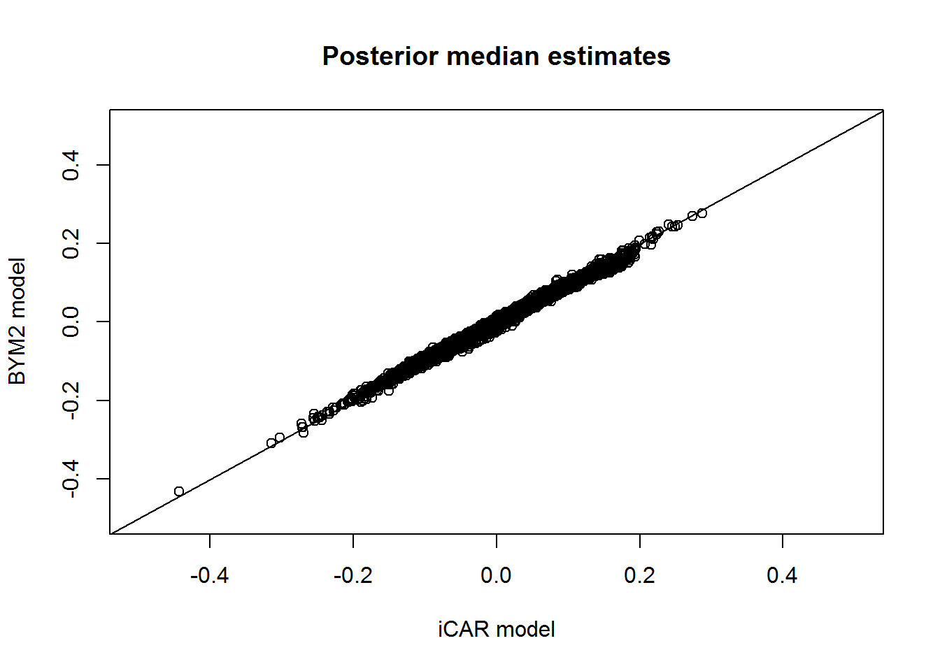
## Model comparisoncompare.DIC <-function(x){data.frame(mean.deviance=x$dic$mean.deviance, p.eff=x$dic$p.eff,DIC=x$dic$dic, WAIC=x$waic$waic,time=x$cpu.used["Total"])}do.call(rbind,lapply(list(iCAR=iCAR.Global, BYM2=BYM2.Global), compare.DIC))
plot(iCAR.Global$summary.linear.predictor$`0.5quant`, BYM2.Global$summary.linear.predictor$`0.5quant`,xlim=c(-0.5,0.5), ylim=c(-0.5,0.5),xlab="iCAR model", ylab="BYM2 model",main="Posterior median estimates")lines(c(-1,1),c(-1,1))
Partition models
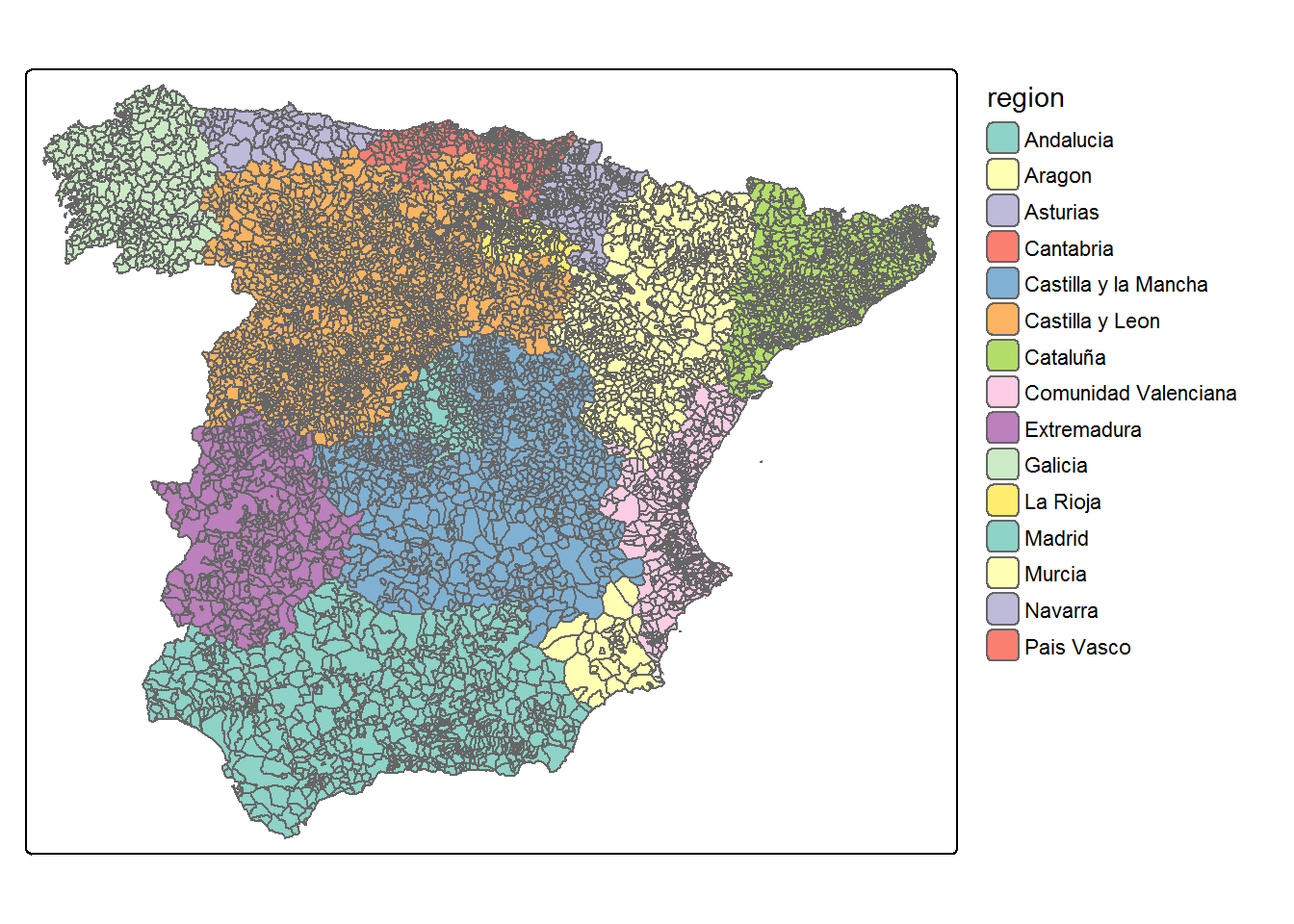
A natural choice for defining the partition of the entire spatial domain could be using administrative subdivisions, such as provinces or states. For our example data, the \(D=15\) Autonomous Regions of Spain are used as a partition of the \(n=7907\) municipalities (Carto_SpainMUN$region variable).
STEP 1: Pre-processing data
STEP 2: Fitting partition (k=0) model with INLA
+ Model 1 of 15
+ Model 2 of 15
+ Model 3 of 15
+ Model 4 of 15
+ Model 5 of 15
+ Model 6 of 15
+ Model 7 of 15
+ Model 8 of 15
+ Model 9 of 15
+ Model 10 of 15
+ Model 11 of 15
+ Model 12 of 15
+ Model 13 of 15
+ Model 14 of 15
+ Model 15 of 15
STEP 3: Merging the results
STEP 1: Pre-processing data
STEP 2: Fitting partition (k=1) model with INLA
+ Model 1 of 15
+ Model 2 of 15
+ Model 3 of 15
+ Model 4 of 15
+ Model 5 of 15
+ Model 6 of 15
+ Model 7 of 15
+ Model 8 of 15
+ Model 9 of 15
+ Model 10 of 15
+ Model 11 of 15
+ Model 12 of 15
+ Model 13 of 15
+ Model 14 of 15
+ Model 15 of 15
STEP 3: Merging the results
STEP 1: Pre-processing data
STEP 2: Fitting partition (k=2) model with INLA
+ Model 1 of 15
+ Model 2 of 15
+ Model 3 of 15
+ Model 4 of 15
+ Model 5 of 15
+ Model 6 of 15
+ Model 7 of 15
+ Model 8 of 15
+ Model 9 of 15
+ Model 10 of 15
+ Model 11 of 15
+ Model 12 of 15
+ Model 13 of 15
+ Model 14 of 15
+ Model 15 of 15
STEP 3: Merging the results
iCAR.k2$cpu.used
 Running  Merging    Total
27.95516 24.37000 52.32516
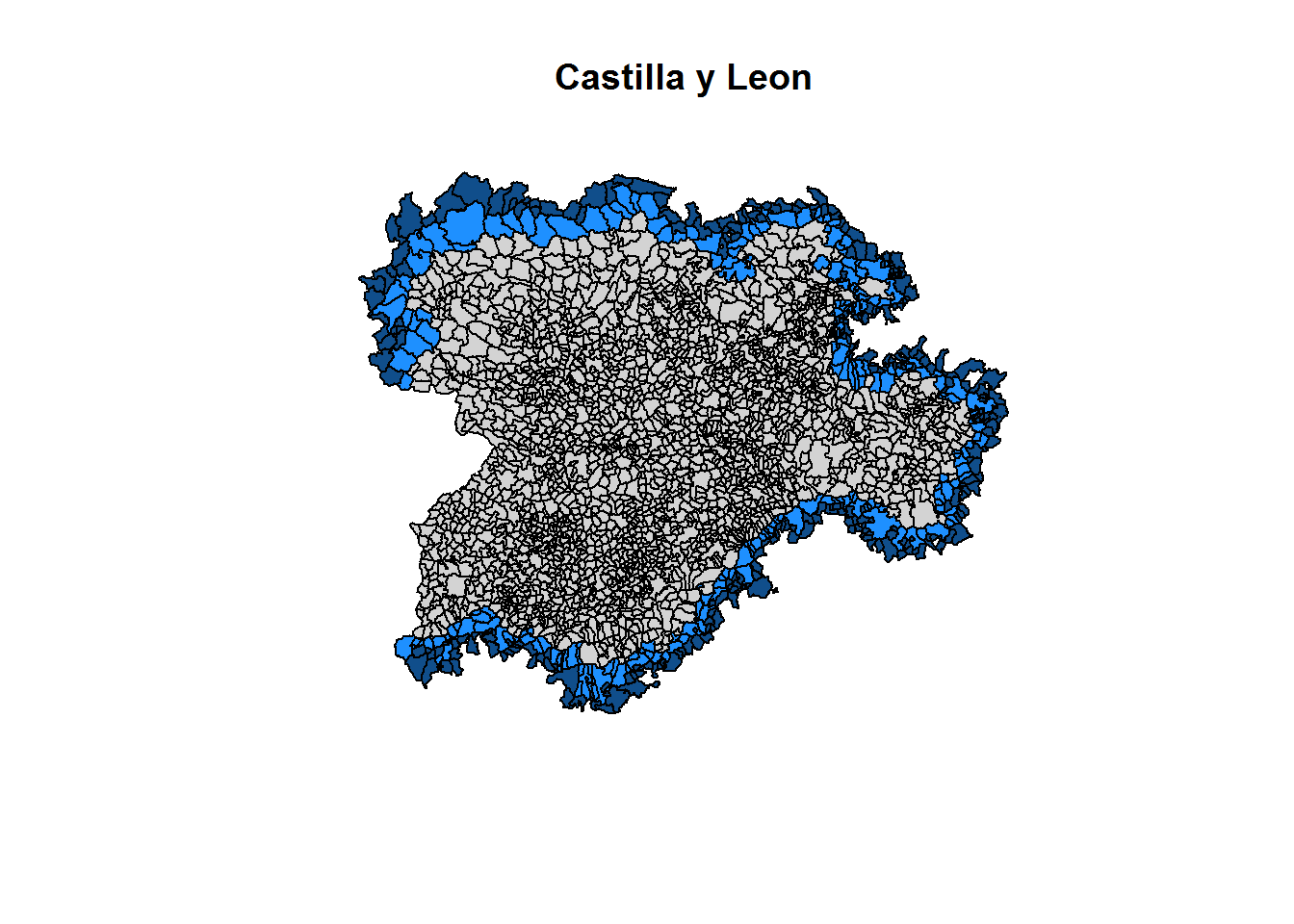
Internally, the divide_carto() function is called to compute the overlapping set of regions \(\{D_1,\ldots,D_{15}\}\) according to the grouping variable ID.group="region". The neighbourhood order to add polygons at the border of the spatial subdomains is controlled by the k argument.
## Compute subdomains for k=0,1 and 2carto.k0 <-divide_carto(carto=Carto_SpainMUN, ID.group="region", k=0)carto.k1 <-divide_carto(carto=Carto_SpainMUN, ID.group="region", k=1)carto.k2 <-divide_carto(carto=Carto_SpainMUN, ID.group="region", k=2)## Plot the spatial polygons for the autonomous region of Castilla y Leon plot(carto.k2$`Castilla y Leon`$geometry, col="dodgerblue4", main="Castilla y Leon")plot(carto.k1$`Castilla y Leon`$geometry, col="dodgerblue", add=TRUE)plot(carto.k0$`Castilla y Leon`$geometry, col="lightgrey", add=TRUE)
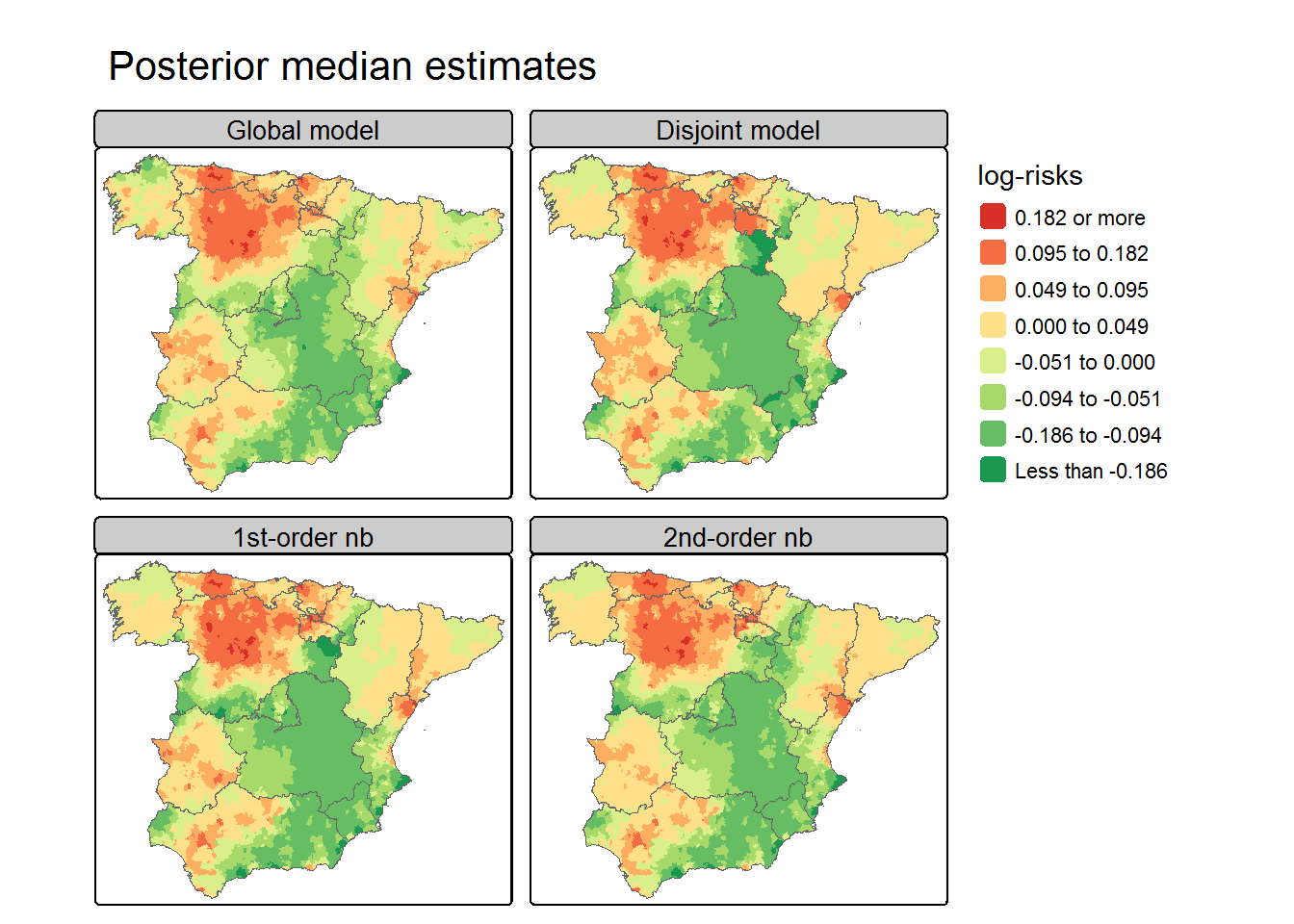
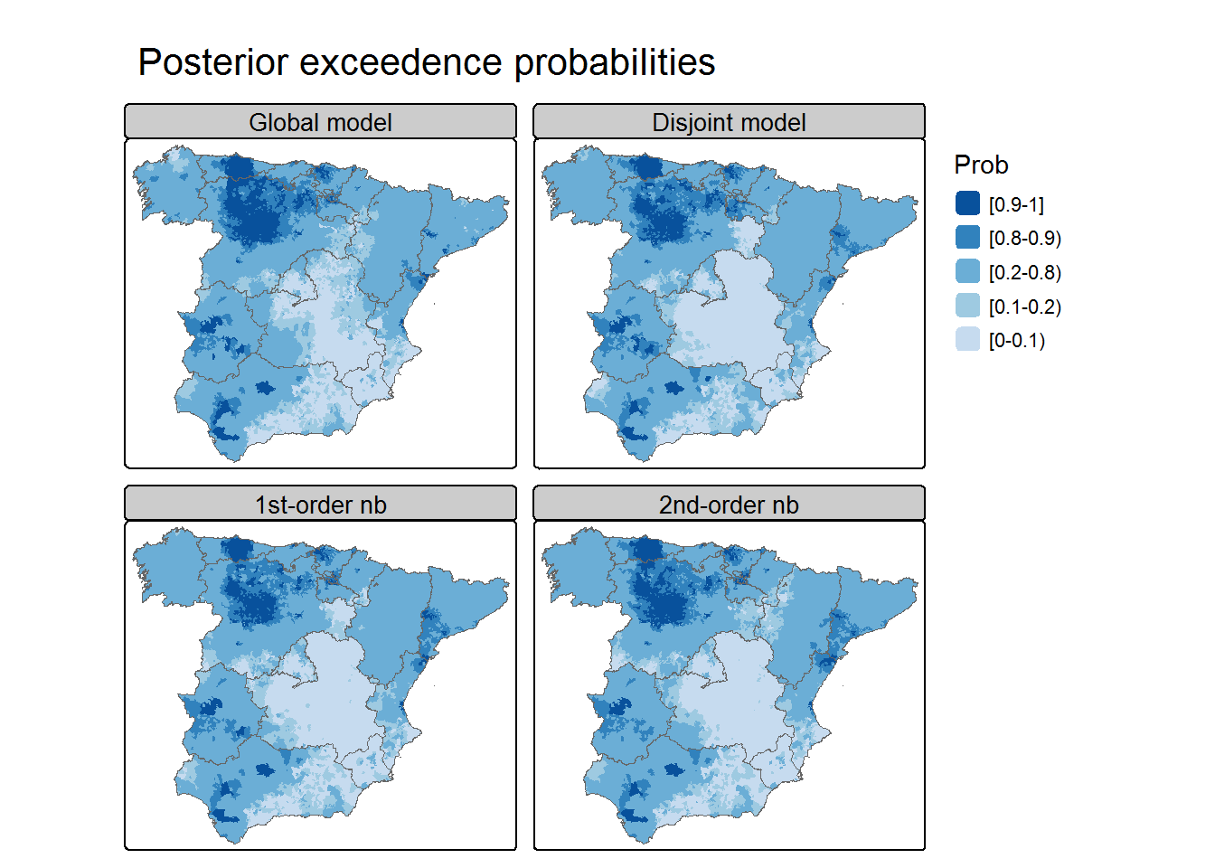
Compare the results
library(RColorBrewer)## Carto object of the Spanish provinces carto.CCAA <-aggregate(Carto_SpainMUN[,"geometry"],list(ID.group=st_drop_geometry(Carto_SpainMUN)$region), head)## Model selection criteriaMODELS <-list(Global=iCAR.Global, k0=iCAR.k0, k1=iCAR.k1, k2=iCAR.k2)do.call(rbind,lapply(MODELS, compare.DIC))
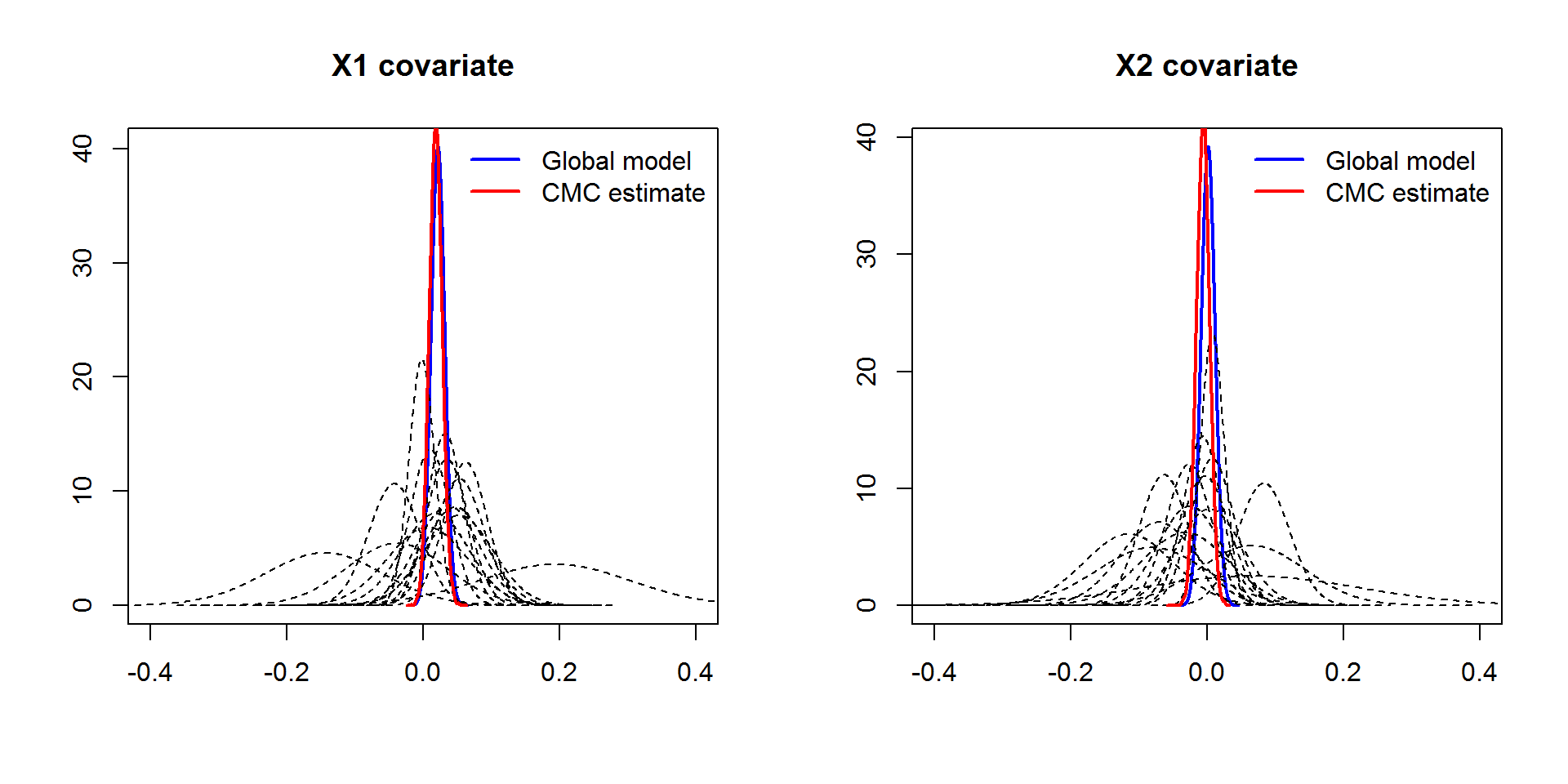
In this second example, we are going to fit a spatial model that incorporates both area-level CAR random effects and a set of explanatory variables, with the aim of comparing the regression coefficient estimates obtained from the global and partitioned models.
For this, we will use the data contained in the Data_MultiCancer object as follows:
## Define the data and the spatial covariates ##data("Data_MultiCancer")head(Data_MultiCancer)
## Define the sf object ##Carto_SpainMUN$obs <-NULLCarto_SpainMUN$exp <-NULLCarto_SpainMUN$SMR <-NULLcarto <-merge(Carto_SpainMUN,data,by="ID")head(carto)
A character vector with the covariate names or the design matrix of the fixed effects can be included through the X=... argument of the CAR_INLA() function:
STEP 1: Pre-processing data
STEP 2: Fitting partition (k=1) model with INLA
+ Model 1 of 15
+ Model 2 of 15
+ Model 3 of 15
+ Model 4 of 15
+ Model 5 of 15
+ Model 6 of 15
+ Model 7 of 15
+ Model 8 of 15
+ Model 9 of 15
+ Model 10 of 15
+ Model 11 of 15
+ Model 12 of 15
+ Model 13 of 15
+ Model 14 of 15
+ Model 15 of 15
STEP 3: Merging the results
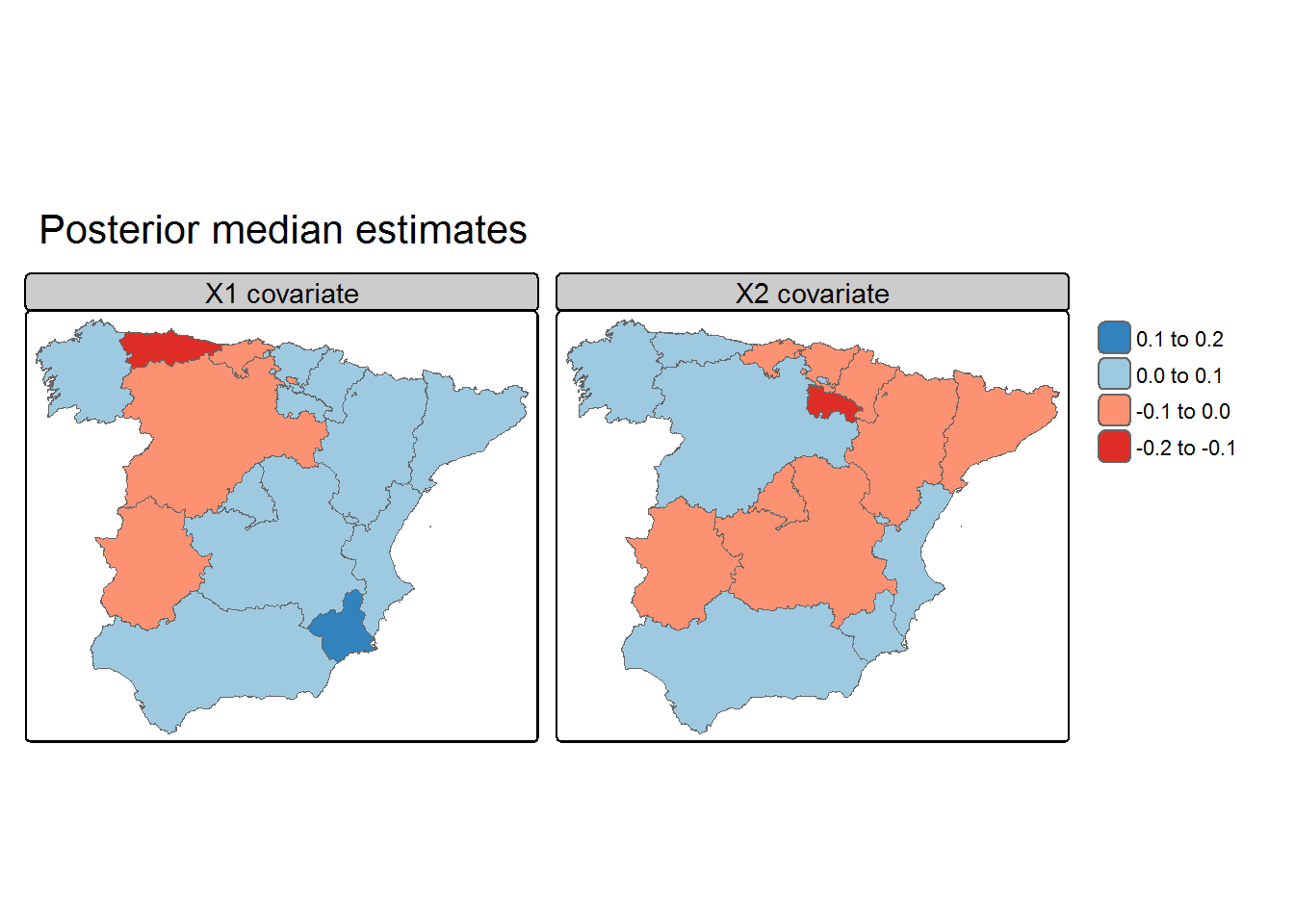
Local and global estimates of the fixed effects
Summary statistics of the posterior marginal estimates for the global model’s fixed effects: