Section 4: Spatio-temporal models for disease mapping
Author
Aritz Adin
Published
Aug 13, 2024
In this lab session we describe how to use the bigDM package to fit spatio-temporal models with conditional autoregressive (CAR) priors for space and random walk (RW) priors for time including space-time interactions (Knorr-Held, 2000; Ugarte et al., 2014) by extending our scalable model’s proposal to deal with massive spatio-temporal data (Orozco-Acosta et al., 2023).
The STCAR_INLA() function
This function allows fitting (scalable) spatio-temporal Poisson mixed models to areal count data, where the linear predictor is modelled as
where \(\beta_0\) is a global intercept, \({\bf x}_{it}^{'}=(x_{it1},\ldots,x_{itp})\) is a p-vector of standardized covariates in the \(i\)-th area and time period \(t\), \(\mathbf{\beta}=(\beta_1,\ldots,\beta_p)^{'}\) is the \(p\)-vector of fixed effect coefficients, \(\xi_i\) is a spatially structured random effect with a CAR prior distribution, \(\gamma_t\) is a temporally structured random effect with a RW prior distribution, and \(\delta_{it}\) is a space-time interaction effect.
These models are flexible enough to describe many real situations, and their interpretation is simple and attractive. However, the models are typically not identifiable and appropriate sum-to-zero constraints must be imposed over the random effects (Goicoa et al., 2018).
Prior distributions for the random effects
Several priors distributions for spatial and temporal random effect are implemented in the STCAR_INLA() function, which are specified through the spatial=... and temporal=... arguments.
For the spatial random effect, the same values as the prior=... argument in the CAR_INLA()function are defined. For the temporally structured random effect, random walks of first (RW1) or second order (RW2) prior distributions can be assumed as follow:
where \(\tau_{\gamma}\) is a precision parameter, \(R_{\gamma}\) is the \(T \times T\) structure matrix of a RW1/RW2, and \(^{-}\) denotes the Moore-Penrose generalized inverse.
Finally, the following prior distribution is assumed for the space-time interaction random effect \(\delta=(\delta_{11},\ldots,\delta_{I1},\ldots,\delta_{1T},\ldots,\delta_{IT})^{'}\)
Here, \(\tau_{\delta}\) is a precision parameter and \(R_{\delta}\) is the \(IT \times IT\) matrix obtained as the Kronecker product of the corresponding spatial and temporal structure matrices (recall that \(R_{\xi}=\textbf{D}_{W}-\textbf{W}\)), where four types of interactions can be considered.
Interaction
\(R_{\delta}\)
Spatial correlation
Temporal correlation
Type I
\(I_{T} \otimes I_{I}\)
-
-
Type II
\(R_{\gamma} \otimes I_{I}\)
-
\(\checkmark\)
Type III
\(I_{T} \otimes R_{\xi}\)
\(\checkmark\)
-
Type IV
\(R_{\gamma} \otimes R_{\xi}\)
\(\checkmark\)
\(\checkmark\)
Table 1: Specification for the different types of space-time interactions
Table 2: Identifiability constraints for the different types of space-time interaction effects in CAR models
Main input arguments
A brief description of the main input arguments and functionalities of the STCAR_INLA() function are described below:
carto: object of class sf or SpatialPolygonsDataFrame. This object must contain at least the variable with the identifiers of the spatial areal units specified in the argument ID.area.
data: object of class data.frema that must contain the target variables of interest specified in the arguments ID.area, ID.year, O and E.
ID.area: character; name of the variable that contains the IDs of spatial areal units.
ID.year: character; name of the variable that contains the IDs of time points.
ID.group: character; name of the variable that contains the IDs of the spatial partition (grouping variable). Only required if model="partition".
O: character; name of the variable that contains the observed number of cases for each areal unit and disease.
E: character; name of the variable that contains either the expected number of cases for each areal unit and disease.
X: a character vector containing the names of the covariates within the carto object to be included in the model as fixed effects, or a matrix object playing the role of the fixed effects design matrix. If X=NULL (default), only a global intercept is included in the model as fixed effect.
W: optional argument with the binary adjacency matrix of the spatial areal units. If NULL (default), this object is computed from the carto argument (two areas are considered as neighbours if they share a common border).
spatial: one of either "Leroux" (default), "intrinsic", BYM or BYM2, which specifies the prior distribution considered for the spatial random effect.
temporal: one of either "rw1" (default) or `rw2``, which specifies the prior distribution considered for the temporal random effect.
interaction: one of either "none", "TypeI", "TypeII", "TypeIII" or "TypeIV" (default), which specifies the prior distribution considered for the space-time interaction random effect.
model: one of either "global" or "partition" (default), which specifies the Global model or one of the scalable model proposal’s (Disjoint model and k-order neighbourhood model, respectively).
k: numeric value with the neighbourhood order used for the partition model. Usually k=2 or 3 is enough to get good results. If k=0 (default) the Disjoint model is considered. Only required if model="partition".
compute.DIC: logical value; if TRUE (default) then approximate values of the Deviance Information Criterion (DIC) and Watanabe-Akaike Information Criterion (WAIC) are computed.
compute.fitted.values: logical value (default FALSE); if TRUE transforms the posterior marginal distribution of the linear predictor to the exponential scale (risks or rates).
inla.mode: one of either "classic" (default) or "compact", which specifies the approximation method used by INLA. See help(inla) for further details.
For further details, please refer to the reference manual and the vignettes accompanying this package.
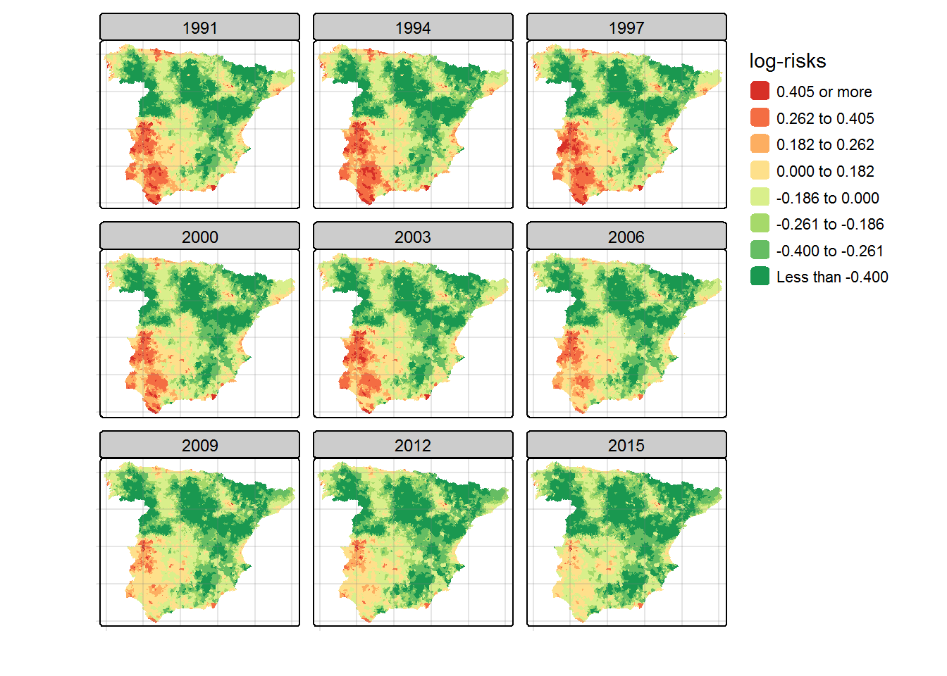
Example: colorectal cancer mortality data during the period 1991-2015
As with multivariate models, both the carto=... and data=... arguments must be included in the STCAR_INLA() function when fitting spatio-temporal models.
In this lab session, the simulated data of lung cancer mortality during the period 1991-2015 included in the Data_LungCancer object will be used as illustration.
library(bigDM)library(INLA)
Cargando paquete requerido: Matrix
Cargando paquete requerido: sp
This is INLA_24.06.27 built 2024-06-27 02:36:04 UTC.
 - See www.r-inla.org/contact-us for how to get help.
 - List available models/likelihoods/etc with inla.list.models()
 - Use inla.doc(<NAME>) to access documentation
library(sf)
Linking to GEOS 3.12.1, GDAL 3.8.4, PROJ 9.3.1; sf_use_s2() is TRUE
library(tmap)
Adjuntando el paquete: 'tmap'
The following object is masked from 'package:datasets':

    rivers
Simple feature collection with 6 features and 5 fields
Geometry type: MULTIPOLYGON
Dimension:     XY
Bounding box:  xmin: 485318 ymin: 4727428 xmax: 543317 ymax: 4779153
Projected CRS: ETRS89 / UTM zone 30N
     ID                                    name           area    perimeter
1 01001                        Alegria-Dulantzi 19913794 [m^2] 34372.11 [m]
2 01002                                 Amurrio 96145595 [m^2] 63352.32 [m]
3 01003                                 Aramaio 73338806 [m^2] 41430.46 [m]
4 01004                              Artziniega 27506468 [m^2] 22605.22 [m]
5 01006                                 Arminon 10559721 [m^2] 17847.35 [m]
6 01008 Arrazua-Ubarrundia (San Martin de Ania) 57502811 [m^2] 64968.81 [m]
      region                       geometry
1 Pais Vasco MULTIPOLYGON (((538259 4737...
2 Pais Vasco MULTIPOLYGON (((503520 4760...
3 Pais Vasco MULTIPOLYGON (((533286 4759...
4 Pais Vasco MULTIPOLYGON (((491260 4776...
5 Pais Vasco MULTIPOLYGON (((509851 4727...
6 Pais Vasco MULTIPOLYGON (((534678 4746...
Global model
The global model, featuring a BYM2 spatial random effect, an RW1 temporal random effect, and a Type IV interaction random effect, is fitted using the STCAR_INLA() function as follows:
## NOT RUN!# Global <- STCAR_INLA(carto=Carto_SpainMUN, data=Data_LungCancer,# ID.area="ID", ID.year="year", O="obs", E="exp",# spatial="BYM2", temporal="rw1", interaction="TypeIV",# model="global", inla.mode="compact")
NOTE: When the number of small areas and time periods increases considerably (as is the case when analyzing count data at the municipality level), fitting spatio-temporal global models with Type II/Type IV interactions becomes computationally very demanding or even unfeasible.
Partition models
For our analysis, we propose to divide the data into the \(D=47\) provinces of continental Spain. To classify the areas into provinces, the first two digits of the ID.area variable is used.
In the code below, we show how to fit the disjoint and 1st-order neigbourhood model with Type II space-time interaction random effect using 4 local clusters (in parallel):
## Model comparisoncompare.DIC <-function(x){ res <-data.frame(mean.deviance=x$dic$mean.deviance, p.eff=x$dic$p.eff,DIC=x$dic$dic, WAIC=x$waic$waic)round(res,2)}MODELS <-list("k=0"=Model.k0,"k=1"=Model.k1)do.call(rbind,lapply(MODELS, compare.DIC))
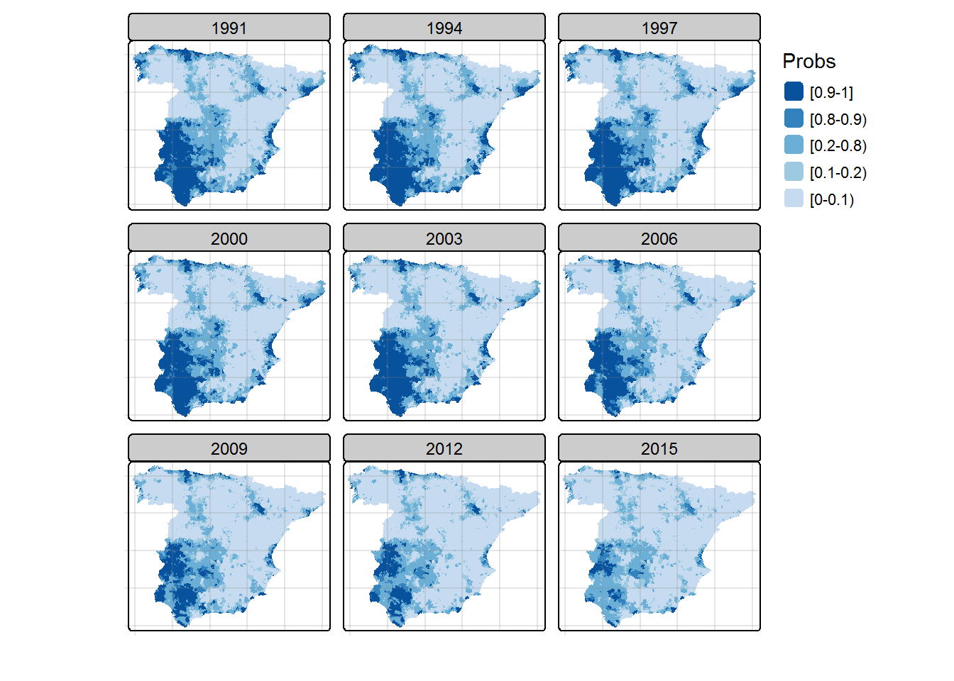
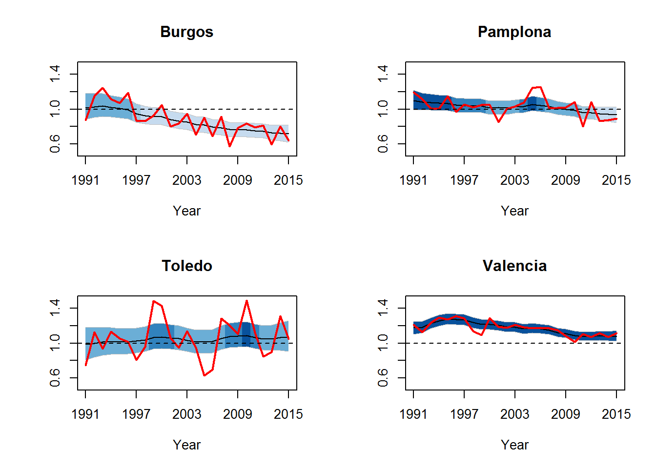
Temporal evolution of mortality risks for some selected municipalities (Pamplona, Valencia and Toledo) and its corresponding 95% credible intervals. The colors used in the bands are associated with the posterior exceedence probabilities represented in the previous maps.